
In this article
I keep coming back to a question that sounds simpler than it is: how much of a file do we actually have to keep?
Look at these bits:
101101101101101101101101
There are 24 of them. But I can describe the pattern as “repeat 101 eight times.” If we agree on a compact way to write that instruction, the instruction might be shorter than the output. For this tiny example, the format and length fields could easily eat the saving. Make the repetition much longer and the idea becomes useful.
That raises a more interesting question. How much information is in the pattern, and how much is in our shared ability to recognize and reproduce it?
This is the thread I want to follow: from ordinary compressed files to learned models, error recovery, video, and possible future hardware. Some boundaries are mathematical. Others are limits of the models, software, and machines we currently know how to build. Telling those apart is where this gets interesting.
Reading route: the first half builds the foundations. “Can recovery help us compress?” connects them to parity and reconstruction. The last sections look at video, text models, and optical computing. The examples are deliberately small enough to check by hand. Select any figure to view it at full size.
Why every file cannot get smaller
Start with a counting exercise, before choosing any compression algorithm.
There are 16 possible four-bit strings. How many shorter binary strings are available to represent them?
| Length | Possible strings |
|---|---|
| Zero bits, the empty string | 1 |
| One bit | 2 |
| Two bits | 4 |
| Three bits | 8 |
| Total shorter than four bits | 15 |
Sixteen distinct inputs cannot fit into fifteen distinct outputs if we require exact recovery. At least two would share a description, and the decoder would have no way to choose between them. In general, there are 2^n n-bit inputs but only 2^n − 1 binary strings shorter than n bits. This is the elementary counting argument behind incompressibility; the table is a worked instance. Grünwald and Vitányi
It still holds if the decoder is an enormous neural network. Fix that decoder and give it an eight-bit seed: there are only 256 seeds, hence at most 256 distinct deterministic outputs. There are 65,536 possible sixteen-bit files. The seed can select a very useful collection of outputs, but it cannot select every possible file of that size.
Additional prompts, model choices, lookup tables, filenames that encode content, or external downloads are additional information. They belong in the accounting.
That is a useful test for a compression claim: what does the decoder already have, and what else must it receive?
Shannon entropy: how surprising is the next symbol?
Shannon entropy describes uncertainty in a probability distribution. For a source that emits symbols with probabilities p(x), its entropy in bits per symbol is:
H(X) = −Σ p(x) log₂ p(x)
The summation means “add this contribution for every possible symbol.” A symbol with probability one contributes no surprise. Unlikely events need more information to identify. We use the convention that a zero-probability term contributes zero. Shannon's source-coding work connects this quantity to achievable average coding lengths. It is a statement about a source and its probabilities, not a universal score attached to any individual file. Shannon, 1948
For an independent binary source, the calculation is particularly approachable:
| Chance of a 1 | Entropy per emitted bit |
|---|---|
| 0% or 100% | 0 bits |
| 10% or 90% | About 0.469 bits |
| 50% | 1 bit |
For example, if successive bits are independent and 90% are ones, the ideal long-run information rate is about 469 bits per 1,000 source bits. That is an average asymptotic target under the stated model; it does not promise a 469-bit archive for every particular 1,000-bit block. Real files also need framing and whatever model information the decoder lacks.
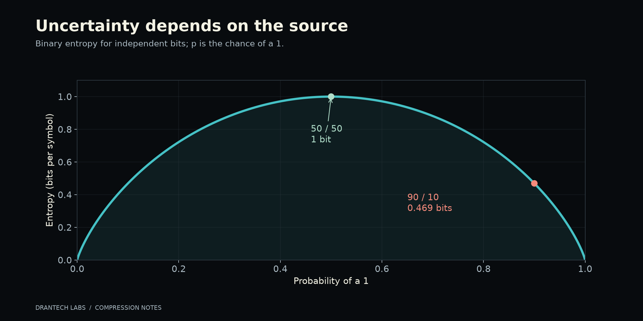
For a discrete source, an optimal prefix code has expected length at least H and less than H + 1 bits per symbol. Coding longer blocks can spread that rounding overhead over more symbols. For dependent sources, the relevant long-run quantity is the entropy rate, incorporating what previous symbols tell us. These conditions matter whenever someone describes an “entropy limit.” CMU source-coding lecture
A histogram can miss the whole pattern
Compare a fair coin sequence with a sequence that alternates forever:
01010101010101010101010101010101
The alternating sequence has equal numbers of zeros and ones. Counting those symbols alone gives one bit of empirical entropy per symbol. Yet after the first bit, the rule determines every subsequent bit.
Formally, choose the first bit fairly and then always flip it. Each individual position has entropy one bit, but a block of n positions contains only one bit of uncertainty: which of the two alternating sequences it is. Its entropy per position therefore tends to zero as n grows. This is a concrete conditional-entropy example, rather than a contradiction of Shannon. Conditional entropy lecture
Later, we will measure the same effect with bytes. The lesson is that a compressor's inability to see a relationship does not make the relationship disappear.
Turning predictions into shorter codes
A simple code can give frequent symbols short representations:
| Symbol | Assumed probability | Code |
|---|---|---|
| A | 1/2 | 0 |
| B | 1/4 | 10 |
| C | 1/8 | 110 |
| D | 1/8 | 111 |
No complete code is the beginning of another, so the decoder knows where each symbol ends. Under these probabilities, the average is 0.5×1 + 0.25×2 + 0.125×3 + 0.125×3 = 1.75 bits per symbol. This is the classic kind of prefix-code example used in source coding. Shannon
Our particular message ABACABAD becomes:
A B  A C   A B  A D
0 10 0 110 0 10 0 111

01001100100111   → 14 bits
Eight symbols using a fixed two-bit alphabet would take 16 bits. Our calculation excludes the shared codebook and message framing. Shipping that table just for this tiny message could make the complete file larger.
Arithmetic coding goes further: it can encode a whole sequence through progressively narrower intervals, rather than allocating a whole number of bits to each individual symbol. A probability model supplies interval proportions; the coder represents which interval contains the actual message. Mahoney, arithmetic-coding explanation
Here is a toy model with P(0)=3/4 and P(1)=1/4. Encode 001, always assigning the lower three quarters of the current interval to zero:
Start      [0, 1)
After 0    [0, 3/4)
After 00   [0, 9/16)
After 001  [27/64, 9/16) = [0.421875, 0.5625)
The binary prefix 1000 describes the interval [0.5, 0.5625), entirely inside the final interval. With the model and the three-symbol length agreed, the decoder can recover 001. Four bits for three source bits is perfectly possible: this short message includes a less likely event and finite-code overhead. This is an interval illustration, not a complete file format.
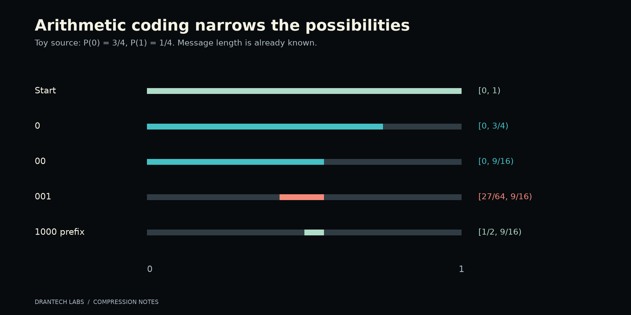
This separation—a model predicts; a coder stores the actual outcome—will matter when we get to LLMs.
Kolmogorov complexity: what is the shortest recipe?
Suppose a file has no obvious repeated text, but a short program can generate it exactly. A general compressor may miss that program completely.
Kolmogorov complexity asks for the length of the shortest program that outputs a particular object on a fixed universal machine. It concerns one specific object, whereas Shannon entropy concerns a distribution. Changing between optimal universal description machines changes complexity by at most a fixed additive constant; on tiny examples, that constant can dominate. In the usual prefix version, written K, programs are self-delimiting: their boundaries can be recognized without a separate length field. Grünwald and Vitányi
There is an awkward catch: we cannot compute this shortest length for arbitrary inputs. Searching programs does not solve the problem, because a shorter candidate that has not finished might run for much longer—or never stop. A compressor that finds a short description provides an upper bound, not a general certificate that no better description exists. Vitányi, 2020
Our repeated 101 has an obvious recipe. The pseudorandom test file later in this article also has a recipe: a particular generator, seed, byte count, and implementation behavior. It may defeat the compressors we test while remaining easy to reproduce from that recipe.
That distinction is worth sitting with. “My compressor cannot shrink this” is a measurement about that compressor. It is not proof that the data has no shorter explanation.
For an actual archive, I would keep a fuller ledger:
Total stored information
  = payload + unshared model/dictionary/program + framing and metadata
This resembles minimum-description-length reasoning: a more elaborate model earns its place only when the shorter description of the data justifies its cost. The most detailed model is not automatically the best total explanation. Grünwald's MDL tutorial
A tiny recipe that takes a year to run also raises a practical issue the byte count cannot settle. We care about decoding time, memory, energy, and whether the required decoder will still be available.
Tries, dictionaries, and remembering what came before
A trie stores keys along paths, sharing the beginnings they have in common. Consider car, cart, cat, and dog:
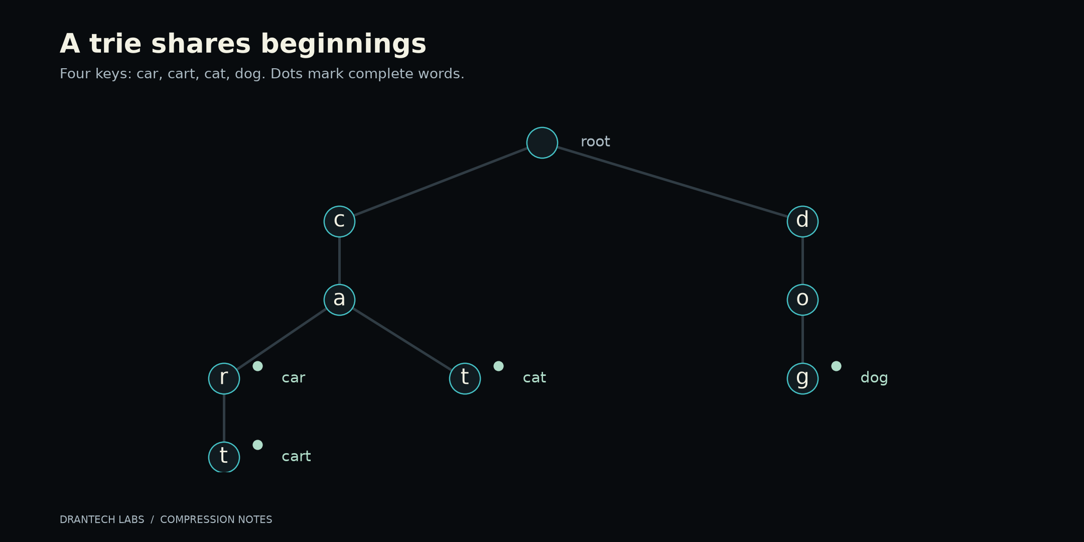
Sharing prefixes is useful for representing and finding related strings. But a basic trie also has nodes, links, and terminal markers; drawing shared letters does not prove the in-memory structure is smaller than a packed list. A trie is a data structure. Its storage layout and the surrounding encoding decide whether it saves bytes. NIST trie definition
A prefix-code tree answers a different question: which bit sequence represents each symbol? The word trie above is organized around the keys themselves. The earlier A→0, B→10 table is organized around codewords. Similar-looking trees can do different jobs.
Dictionary compressors exploit repeated material too. In a conceptual LZ-style representation:
Input:    101101101101
Recipe:   literal 101; copy 9 symbols from 3 positions back
The copy can overlap its own growing output: each newly reconstructed symbol becomes available for the next step. The distance and length still cost bits. This is a conceptual back-reference, not a claim that a particular codec compresses this twelve-bit toy. Zstandard's format specifies concrete literals, match lengths, and offsets. RFC 8878
LZW takes another route, building a dictionary of phrases and sending dictionary codes. Princeton's teaching implementation illustrates that construction and its decoding counterpart. A trie can help implement dictionary lookup, but it is not synonymous with LZW. Princeton LZW implementation
PAQ, Zstandard, and Brotli
These names represent different engineering choices, not rungs on one universal quality ladder.
| Family | What it does | What to pay attention to |
|---|---|---|
| PAQ | Mixes contextual predictions and uses them in arithmetic coding. | Model complexity, memory, time, and the particular PAQ variant. |
| Zstandard / Zstd | Combines repeated-sequence matches with entropy coding; its format uses Huffman and finite-state entropy coding. | Compression level, latency, memory, data type, and dictionary use. |
| Brotli | Combines LZ77-style references, Huffman coding, context modeling, and a built-in dictionary with transforms. | Quality setting, input type, window, and the cost of encoding. |
The original PAQ1 paper describes several predictors looking at different kinds of context, combined to estimate the next bit before arithmetic coding. The wider PAQ project contains many descendants and variants. Its value here is the idea: several imperfect views of the same data may produce a better probability estimate together. It is not one timeless “best compressor.” Mahoney's PAQ1 paper, PAQ project
Zstandard's literals can be Huffman-coded, while sequence codes use finite-state entropy coding. Its project also supports training dictionaries on representative samples, useful when small related records do not provide much history on their own. Those dictionaries must be available to the decoder. RFC 8878, Zstandard project
Brotli's static dictionary is built into the format, with transformations that can produce related words or fragments. It is shared prior knowledge, paid for in the decoder rather than retransmitted for every file. That is different from training a custom dictionary for a particular collection. RFC 7932
A small experiment: the pattern matters
For this article, I generated three files, each exactly 262,144 bytes (256 KiB):
- Periodic: the byte values 0 through 255, repeated 1,024 times.
- Telemetry: synthetic JSON lines with repeating field names, cycling sensor/state values, and changing counters and temperatures, truncated to the same byte length.
- Pseudorandom: bytes from Python's deterministic generator, using seed
20261011.
These are deliberately artificial examples. They are not a representative benchmark suite or a test of cryptographic randomness.
| Input | Zstd level 3 | Zstd level 19 | Brotli quality 5 | Brotli quality 11 |
|---|---|---|---|---|
| Periodic | 291 B | 292 B | 260 B | 218 B |
| Telemetry | 9,266 B | 7,064 B | 6,786 B | 4,370 B |
| Pseudorandom | 262,159 B | 262,159 B | 262,149 B | 262,149 B |
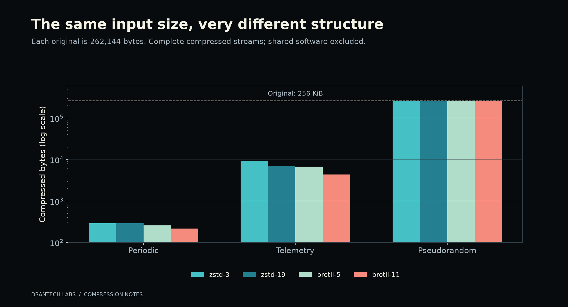
The periodic input has exactly eight bits of byte-histogram entropy per byte. Every byte value appears equally often. Yet Brotli quality 11 represented the whole file in 218 bytes. The histogram ignored the order; the compressor found the repeated sequence. There is no conflict with an entropy-rate limit.
The pseudorandom input grew slightly in all four cases. That does not establish high Kolmogorov complexity: the saved generation script is itself a short recipe for it. It shows that these codec configurations did not find useful savings in this particular output.
One small detail is revealing: Zstd level 19 produced one more byte than level 3 on the periodic input. A higher setting is not a promise of a strictly smaller result for every possible file.
The experiment used libzstd 1.5.7, Python's zstandard binding 0.25.0, and Brotli 1.2.0. Sizes include the returned compressed streams but exclude codec software. There was no trained dictionary; Brotli's standard dictionary remains part of its decoder. The script and full results with hashes are available below. PAQ was not benchmarked.
Lossless, lossy, and generated: what did we promise to recover?
For this article, lossless means recovering the exact original byte sequence. A prettier approximation does not qualify.
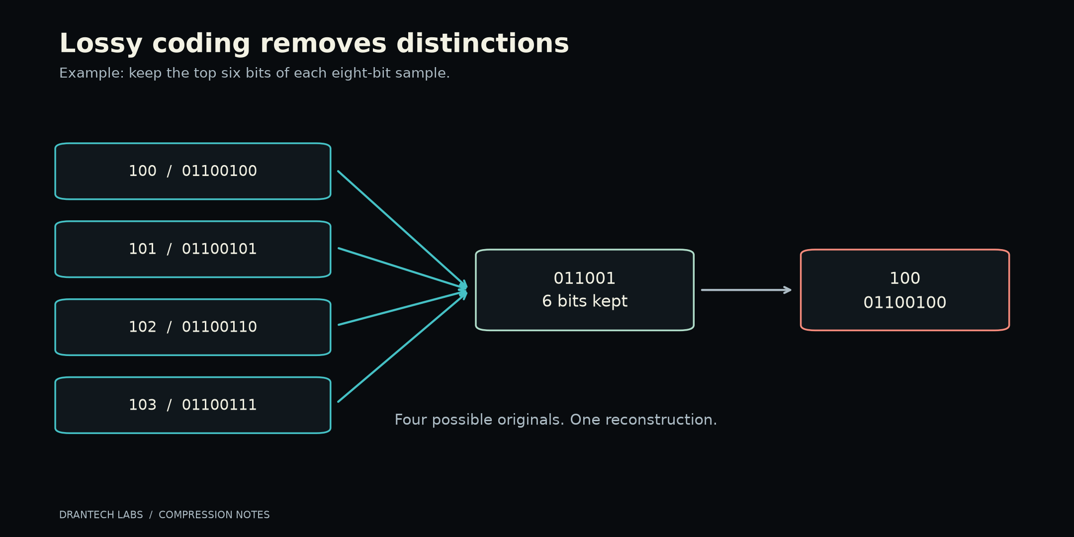
Lossy coding permits some distinctions to disappear. Here is a deliberately crude quantizer: divide an eight-bit sample by four, discard the remainder, and reconstruct by multiplying by four.
Original       Kept six bits       Reconstructed
100 = 01100100     011001           100 = 01100100
101 = 01100101     011001           100 = 01100100
102 = 01100110     011001           100 = 01100100
103 = 01100111     011001           100 = 01100100
Two low bits per sample are gone. All four inputs now share one stored representation. No decoder can determine which original value we had from those six bits alone. This is a worked many-to-one mapping, not a model of the full JPEG or video pipeline.
Rate-distortion theory studies the tradeoff between bits and a specified measure of error. But numerical closeness and perceptual realism are different goals. Blau and Michaeli formalize a three-way relationship between rate, distortion, and perception: a visually convincing result need not be the closest reconstruction of the particular original. Blau and Michaeli, 2019
That matters with generative reconstruction. If a decoder invents plausible grass texture, skin detail, or lettering, it may produce something attractive without restoring what the camera recorded. I would want that distinction made explicit for any scientific image or evidentiary record.
A generator can also be exact. Our repeating-bit recipe is one. But for a complex generator, “save the seed” only works if the target actually belongs to its possible outputs and the required model, settings, and execution behavior are fixed. The counting argument still applies. The distinction is whether we can reproduce the original, or merely produce something that looks as though it could have been the original.
In what sense are LLMs compression?
There is a precise connection, and a looser metaphor. They should not be mixed together.
An autoregressive language model estimates probabilities for the next token given preceding tokens. Those probabilities can drive an arithmetic coder: likely continuations get cheaper descriptions; unexpected continuations cost more. The decoder uses the same probabilities and the coded bits to recover the actual tokens. Delétang and colleagues study this connection directly in Language Modeling Is Compression. Delétang et al., 2023/2024
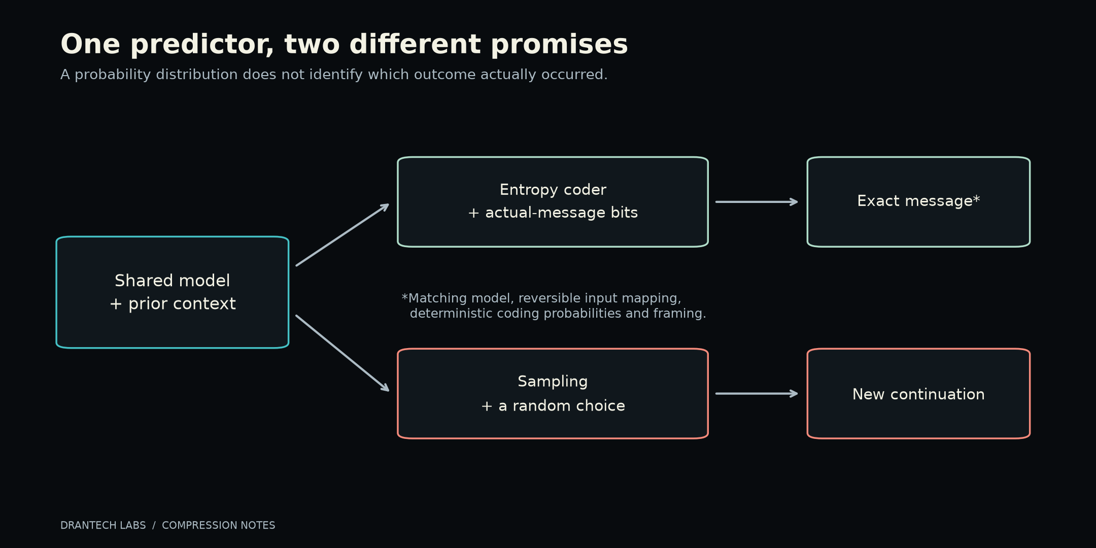
This is more than an analogy. Fabrice Bellard's experimental ts_zip uses a pretrained language model for text compression. Its documentation explicitly discusses reproducibility and deterministic inference. NNCP explores neural compression with learning during compression. They are useful examples of implementations to inspect, not evidence that every LLM is a practical archive format. ts_zip, NNCP
For a byte-exact design, I would ask concrete implementation questions: Is tokenization reversible for every accepted input? Are model weights and vocabulary identified? Does the probability-to-integer conversion agree at both ends? How are termination and model versions stored? Can another machine decode it?
Those last questions are serious. Ballé, Johnston, and Minnen show that small numerical differences between encoder and decoder probability calculations can break entropy decoding; their integer-network approach addresses cross-platform consistency. A vaguely similar prediction is not sufficient. Integer Networks, 2019
The looser claim is that training compresses regularities from a large corpus into model parameters. That can be a useful description of learning, but the parameters are not generally a reversible archive of the corpus. An ordinary generated answer is not an exact decompression operation. The paper's lossless-coding experiments provide a specific, testable connection; they do not make every use of a chatbot lossless. Language Modeling Is Compression
Who pays for the shared model?
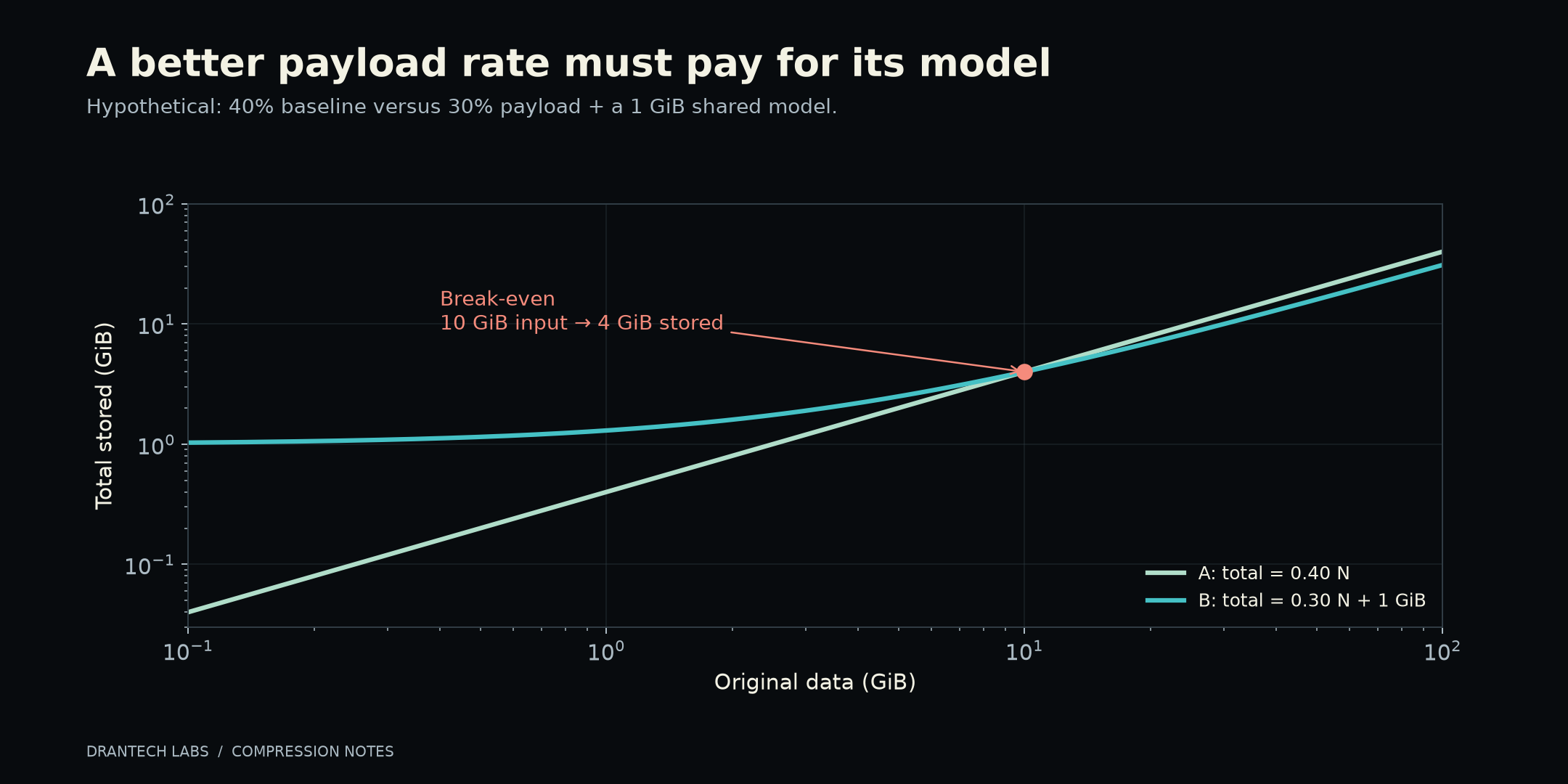
Here is a hypothetical comparison, with deliberately invented rates:
Codec A: compressed data occupies 40% of its original size.
Codec B: compressed payload occupies 30%, plus a 1 GiB model.

Total A = 0.40 N
Total B = 0.30 N + 1 GiB
Break-even: N = 10 GiB
Below 10 GiB, B's better payload rate loses on this simplified total-storage measure. Above it, the model cost has been shared across enough data to pay off. We have ignored other overheads and assume the same rates across all N; this is accounting, not a performance forecast.
The question I find interesting is whether a small, specialized model could capture enough structure to be useful without carrying a general model's cost. That is an experiment to run, with conventional compressors included as baselines.
Can recovery help us compress?
Yes, under the right assumptions. But first we need to separate two uses of redundancy.
Ordinary parity buys recoverability
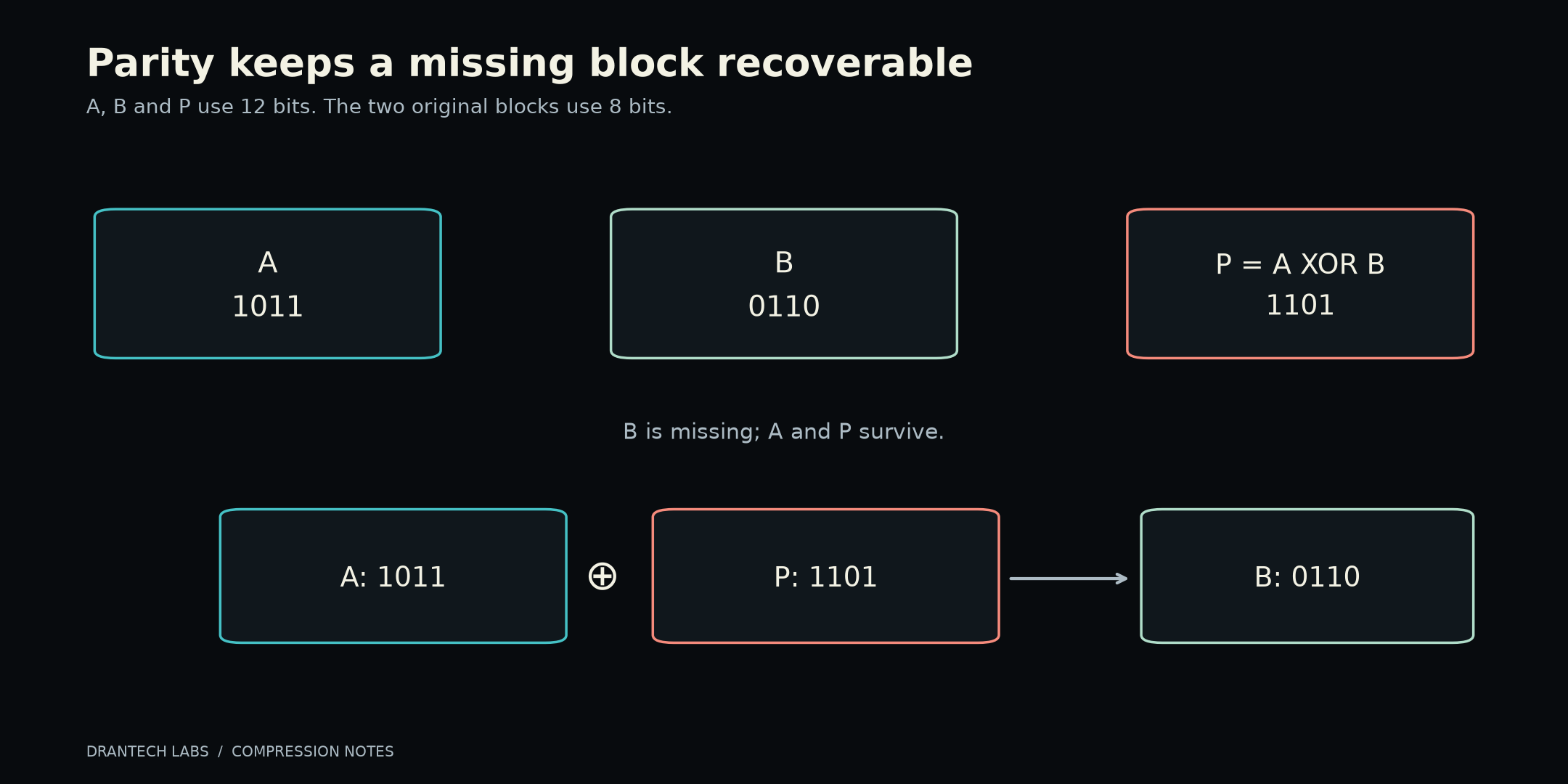
XOR is a bitwise operation: equal bits produce zero, different bits produce one. Take two four-bit blocks:
A       1011
B       0110
A XOR B 1101   ← parity block P
Store A, B, and P and we now have twelve bits instead of eight. That is 50% more storage, not compression.
But if B is missing and we know it is the missing block, we can reconstruct it:
A XOR P = 1011 XOR 1101 = 0110 = B
The same works for A if B and P survive. Keep P alone and there are still sixteen possible (A, B) pairs: each possible A determines a corresponding B. The parity block has not secretly preserved eight arbitrary bits in four.
A single even-parity bit makes the total number of ones even. A flipped bit changes that parity, so the check detects an odd number of flips but misses an even number. Detection does not automatically identify the damaged position. Hamming's work develops codes that can locate and correct errors under defined conditions. Hamming, 1950
More powerful erasure codes extend the recovery idea. The Reed–Solomon schemes specified in RFC 5510 can recover k source symbols from any k of their encoded symbols. Additional repair symbols provide tolerance for missing ones. They do not make the original unconstrained information disappear. RFC 5510
This can still reduce a system's total storage compared with its chosen replication scheme. In our toy example, two complete copies of A and B take sixteen bits; A, B, and P take twelve. Those layouts have different failure properties, so that arithmetic alone is not a deployment recommendation. It shows why storage efficiency through recovery coding and source compression are useful but distinct ideas.
Three check bits can identify a seven-bit message—with help
Now give the receiver something valuable: a related seven-bit string Y. The sender has X. We promise that X and Y differ in at most one position.
Position:  1 2 3 4 5 6 7
X:         1 0 1 1 0 0 1
Y:         1 0 1 1 1 0 1
                    ↑
                 difference
Instead of sending all seven bits of X, send three parity checks, called its syndrome. Define them as:
p1 = XOR of positions 1, 3, 5, 7
p2 = XOR of positions 2, 3, 6, 7
p4 = XOR of positions 4, 5, 6, 7

Write the syndrome as p4 p2 p1.
For X, those checks produce 001. For Y, they produce 100. The receiver XORs the syndromes:
001 XOR 100 = 101 = position 5
Flip position five in Y and we recover X exactly. If the difference were 000, the promise would imply that no bit needed changing.
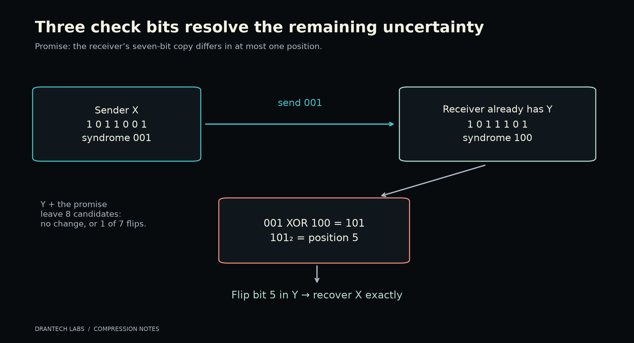
Why three bits? Given Y and our promise, there are only eight candidates for X: Y itself or one of its seven single-bit changes. Three bits distinguish eight possibilities. We have compressed the remaining uncertainty, not seven arbitrary bits without assistance. If we first have to send Y just to make this work, its seven bits also count: seven plus three is worse than sending X directly. The benefit depends on genuinely available side information.
If two positions differ, this decoder can choose a wrong correction. A real system needs a justified model of the differences, a way to handle failures, and suitable integrity checking. The toy demonstrates the principle under a strict promise; it is not a production reconciliation protocol.
There is a deeper theorem behind the broader idea. Slepian and Wolf showed how correlated sources can be coded separately and decoded together. With suitable discrete memoryless source assumptions and long blocks, a source can be communicated at rates approaching its conditional entropy H(X|Y) when Y is available to the decoder, with decoding error probability tending to zero. That is an asymptotic statistical result, distinct from our small example's exact one-error promise. Slepian and Wolf, 1973
Using coding syndromes for distributed compression is an established research direction; Pradhan and Ramchandran's DISCUS work is explicitly about that connection. The exciting part is that the encoder need not always possess the decoder's side information to exploit its existence. Authors' DISCUS publication record
This suggests a practical question for research: how much are we retransmitting because our systems fail to use related information already present at the receiving end?
Reconstructing from fewer measurements
Compressed sensing asks a related question at acquisition time. If a signal is sparse—having few nonzero coefficients in a suitable representation—appropriate measurements can sometimes recover it from fewer observations than a generic signal would require. Candès, Romberg, and Tao establish exact-recovery results under explicit sparsity and measurement conditions, not for arbitrary signals. Robust Uncertainty Principles
Here is a much simpler illustration of how assumptions help. We know an eight-position vector contains exactly one positive integer value and everything else is zero:
Position:  1 2 3 4 5 6 7 8
Value:     0 0 0 0 3 0 0 0

Measurement 1: sum of values              = 3
Measurement 2: sum of position × value    = 15

Nonzero value = 3
Its position  = 15 / 3 = 5
Two measurements recover the vector under that promise. Change the promise to permit two arbitrary nonzero values and the same two sums need not identify it uniquely.
Also, two measurements are not two bits. Their numerical ranges, precision, noise, and encoding cost all matter. This toy is a demonstration of constrained reconstruction, not a practical compressed-sensing algorithm or proof of a bit-rate advantage. Work on stable recovery explicitly addresses imperfect measurements under further conditions. Stable Signal Recovery
The common thread is now visible: a dictionary, a predictive model, a correlated copy, or a sparsity assumption can supply structure. The remaining message tells us which member of the allowed set actually occurred.
Video: better predictions, cheaper corrections
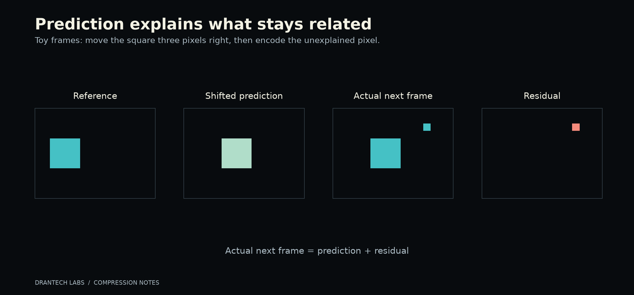
Think of a square moving across a plain background. If the decoder already has a reference frame, a motion description can help predict the next one. Then it needs the information that the prediction failed to explain—the residual—plus the relevant coding decisions. Real block-based video formats include prediction, transforms, quantization, and entropy decoding rather than simply saving differences between raw frames. AV2 decoding specification
Where the field stands on October 11, 2026
AV2 is already a final specification. AOMedia lists version 1.0.0 and matching reference software dated May 28, 2026. Its January 2026 “v13” was a working draft and is superseded; the larger-looking version number does not make it newer. Official AV2 release index
A specification is only part of the route to everyday use. AOMedia's July 27, 2026 implementer discussion distinguishes the reference software from optimized implementations and the hardware support needed for wider deployment. I would not turn a reference-code comparison into a promise about playback efficiency on a particular phone. AOMedia implementation update
Beyond VVC remains a development program. ITU's July 28, 2026 report describes the call for proposals, evaluation planned for January 2027, and a target for a future standard by 2029. These are stated plans, not a shipping codec or a guaranteed completion date. ITU: Beyond VVC
Learned coding is also reaching standards and practical research. JPEG's February 19, 2025 announcement reports approval of the JPEG AI text for publication as an International Standard. That is learned image coding, not a new video format. JPEG committee announcement
For video, the CVPR 2025 DCVC-RT paper is interesting because it tackles practical bottlenecks, including memory traffic and operational overhead, rather than treating arithmetic count as the whole problem. It also addresses cross-device consistency. Its reported speed and compression results belong to its test setup; they do not establish a universal winner over production encoders. Jia et al., 2025
I expect useful comparisons to ask more than “how many bits?” How much power does decoding require? How quickly can playback start? What happens at a scene cut? Which details are preserved? Can a low-cost device keep up? Better compression that changes those tradeoffs could matter well beyond making the same stream a little smaller.
What could a better text compressor discover?
Text offers several kinds of structure at once: recurring bytes, words, grammar, document templates, subject matter, and relationships across long distances. The interesting question is which of those a model can exploit cheaply and reliably.
There are theoretical results for specific model classes. The context-tree weighting method combines predictions over a class of finite-memory tree sources and gives coding guarantees within that setting. Its universality is not a promise to find the shortest program for every possible text. The model class is part of the claim. Willems, Shtarkov, and Tjalkens, 1995
At the more ambitious end, algorithmic probability considers explanations in terms of programs, favoring shorter descriptions. Its fully general form is not computable. It offers a way to think about prediction, without giving us an implementable optimal compressor for arbitrary data. Grünwald and Vitányi, algorithmic probability discussion
My research interest would be in manageable combinations: exact phrase reuse for repetitive passages, a compact model for domain structure, and a conventional fallback when the model helps too little. The experiment would need to count model storage, test genuinely held-out material, and verify every decoded byte. This is a proposed direction, not a claim of a new result; existing context mixing and neural compressors are essential baselines.
One possibility worth testing is that a narrow model of a company's repeated document formats beats a much larger general model on the company's actual workload. Another is that the simpler dictionary already captures nearly everything worth capturing. Both answers would be useful.
Could optical computing help?
Possibly, by changing the cost of computation. Light does not create a new exception to information theory.
Research has demonstrated optical and hybrid optical-electronic matrix multiplication for neural processing. Meng and colleagues' 2025 work investigates a digital–analog hybrid design to address precision and noise. It is evidence for a computing component, not a demonstration of a general-purpose optical compressor. Meng et al., 2025
A 2026 photonic-memory study investigates integrating memory with photonic computation, addressing the expense of moving data and repeatedly converting between electrical and optical representations. Its neural-processing demonstrations should not be mistaken for end-to-end compression measurements. Neuromorphic photonic memory, 2026
The following is my inference from those capabilities: if a useful compression model spends much of its time on suitable matrix operations, a future photonic accelerator might reduce that part of its compute cost. Whether it improves the complete codec would depend on precision, model storage, conversion overhead, utilization, and the rest of the pipeline.
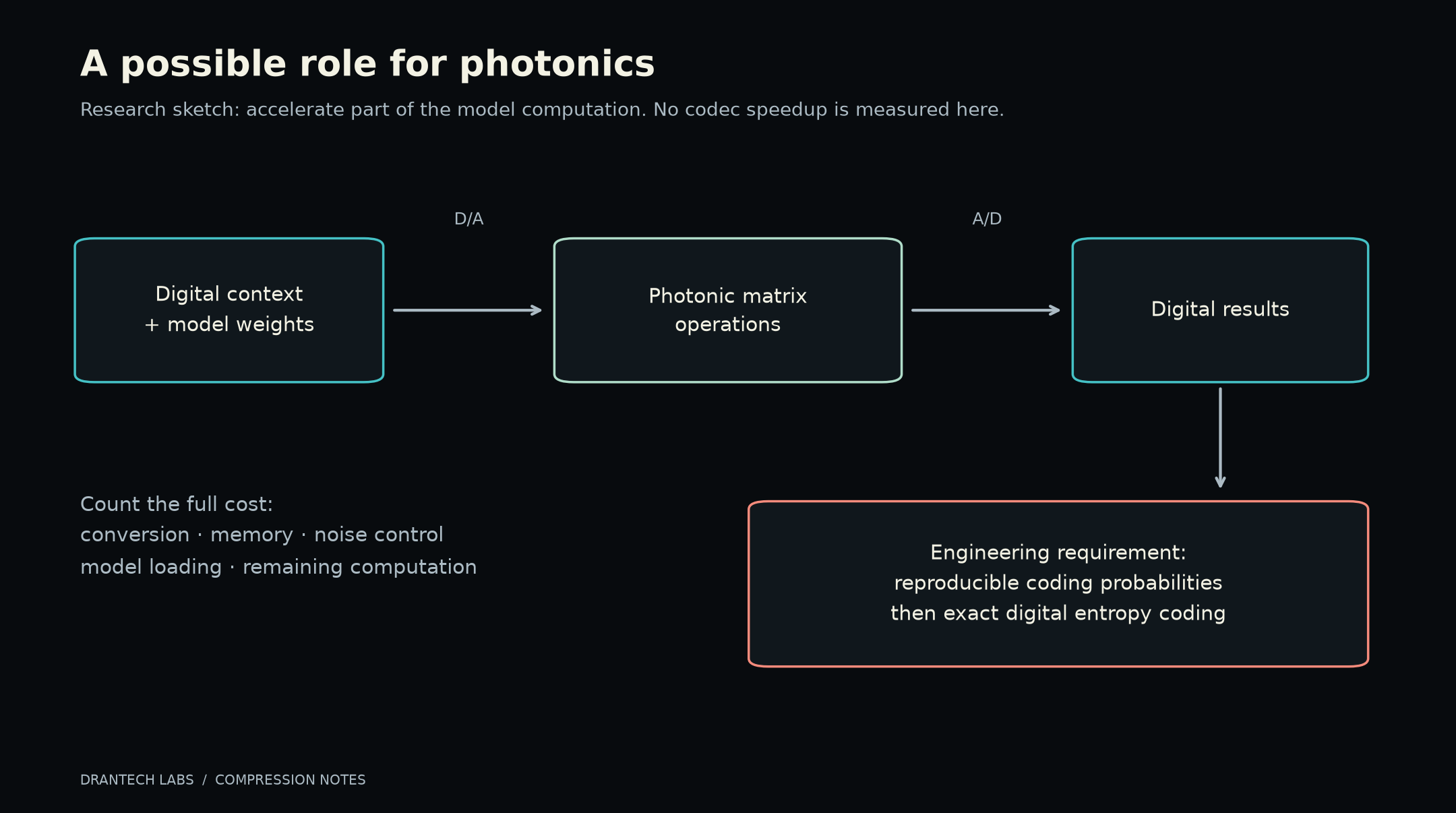
Exact entropy decoding makes reproducibility especially demanding. A faster approximate probability calculation is not useful if the two ends disagree and the archive becomes unreadable. The numerical-consistency issue documented in learned compression still applies; photonic noise would have to be handled within an explicit design. Integer Networks
I would start by measuring the entire proposed system, including data movement and electrical–optical conversions. Otherwise, a spectacular matrix-operation figure could hide a disappointing compressor.
The questions the limits leave open
The counting limit is firm. The shortest-program problem is not generally computable. Neither statement tells us that the compressors we use today have found every useful relationship in the data we care about.
The most promising question may be less “how do we pack these bits more tightly?” and more “what would let the receiver reconstruct them with less new information?”
For Drantech Labs, I would turn that into a few specific investigations:
| Question | An experiment that could answer part of it |
|---|---|
| How much structure do ordinary codecs miss in a narrow workload? | Compare dictionaries, small predictors, and existing codecs on held-out data, including all model bytes. |
| When is decoder-side information worth exploiting? | Measure syndrome-based reconciliation on controlled differences, including failure detection and recovery traffic. |
| Can stronger prediction pay for its own compute? | Report total size, latency, memory, and energy together; include a model-free baseline. |
| Which reconstructed details are trustworthy? | Separate exact recovery from perceptual generation, and test how errors affect the intended use. |
| Can a compressed representation remain usable years later? | Package decoder versions and dependencies, then test recovery on a separate machine. |
These are proposed experiments, not completed Drantech results. The synthetic size measurements earlier are the only new codec measurements reported here.
Even an ordinary-looking improvement can have consequences when repeated across enough data. Consider a hypothetical workload storing 100 TB: a real 10% reduction would save 10 TB before replication and overhead. Whether it also saves money or energy depends on the system and the cost of getting that reduction. A smaller result is an invitation to measure the rest, not permission to assume it.
More surprising improvements could change what is practical to keep, transmit, or process locally. A useful model shared once might make subsequent communication much cheaper. Better acquisition could avoid collecting some redundant measurements in the first place. Better recovery coding could change the storage cost of resilience. Those possibilities come with dependencies: the shared model, the signal assumptions, the decoder, the confidence that recovery is exact.
The question I want to investigate is this:
How much of what we call information is a relationship we have not yet learned to use—and what would become possible if we could use it reliably?
Sources and reproducibility
Research checked October 11, 2026. Links beside the claims lead to original papers, specifications, author implementations, and university teaching material. The explanations and proposed experiments are distinct from original research findings. All eleven figures were made for this article; select any figure to view it at full size.
The synthetic size experiment is the only new codec measurement reported here. Its four configurations all recovered the exact original bytes. The accompanying calculation checks verify the binary examples, including all 1,024 allowed cases in the syndrome example. No PAQ, LLM, video, optical, speed, or energy benchmark was performed.
Download the compression experiment script, measured results and hashes, worked-example verification script, and calculated results. These are plain-text files you can inspect before running anything.
To reproduce the experiment, save the scripts as tools/measure.py and tools/check_examples.py, removing the download's .txt suffix, and create an adjacent evidence directory. The recorded environment used Python 3.14.7, zstandard 0.25.0 with libzstd 1.5.7, and Brotli 1.2.0. In a Python environment with those codec bindings installed, run:
python3 tools/measure.py
python3 tools/check_examples.py
The scripts write their results into evidence. Different codec versions can produce different compressed bytes, so compare versions and input hashes before interpreting a difference. The three inputs are generated locally; no customer data or external dataset is required.